

Chandrayaan-4 Preliminary Site Analysis: What the Data Actually Shows
Building a 29 cm DEM from raw stereo, aligning it to LOLA, and validating ISRO's landing site selection — one criterion at a time

In January 2026, ISRO’s Space Applications Centre published a two-page abstract at the 57th Lunar and Planetary Science Conference describing five candidate landing sites on Mons Mouton for the Chandrayaan-4 mission (Amitabh et al., LPSC 2026, #1198).
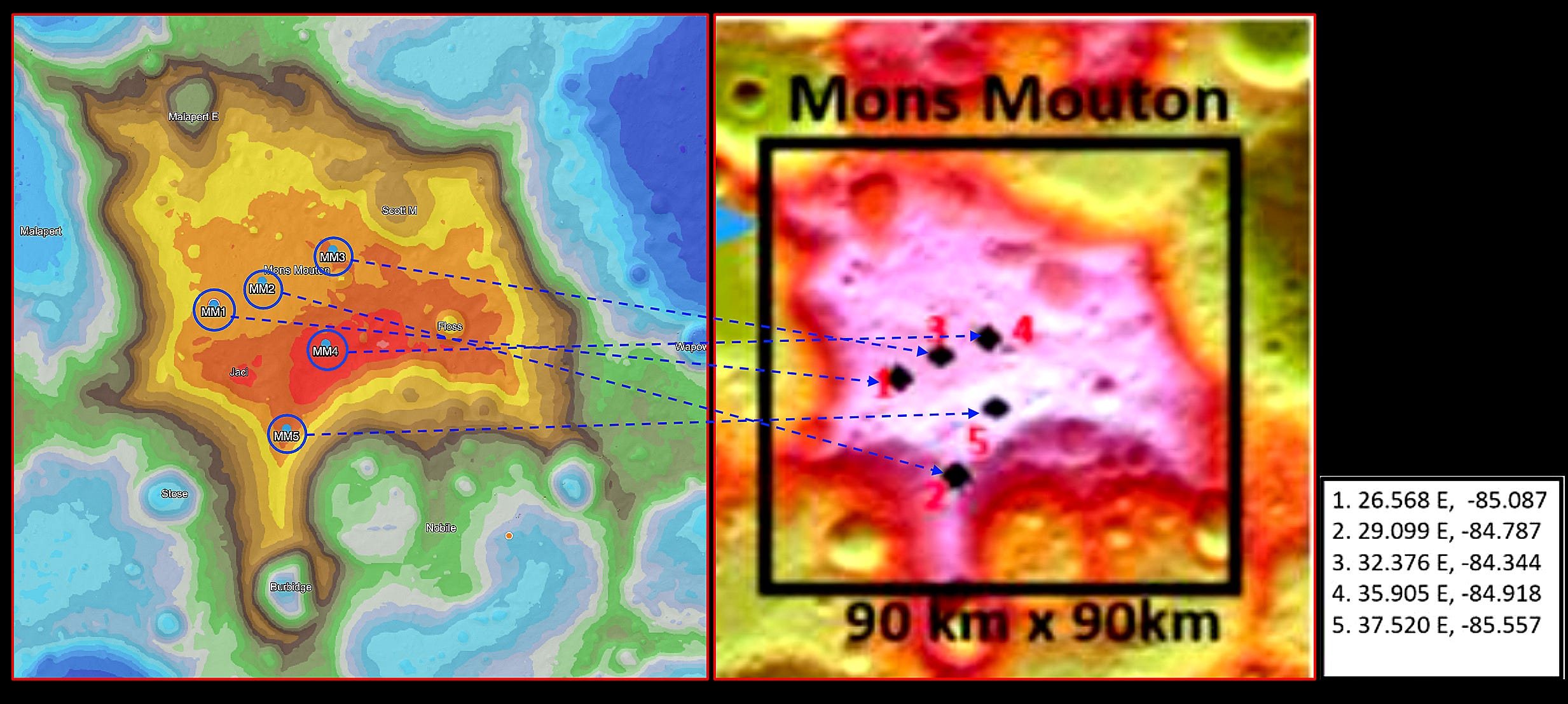
Based on engineering constraints, MM-4 was identified as the primary landing location for Chandrayaan-4. The site was evaluated for slope safety, boulder hazards, and sunlight availability, and a 1 km × 1 km area within it was found to have
the least hazardous terrain. The final landing site was selected using the following criteria:
Slope <= 10°
Boulders < 0.32 m diameter (detection limit because of OHRC pixel resolution for the acqusitions)
Crater and boulder distribution
Sunlit for at least 11–12 days per lunar cycle
Local terrain features don’t shadow the site for prolonged durations
Distribution of safe 24 m × 24 m grids inside the 1 km × 1 km landing area
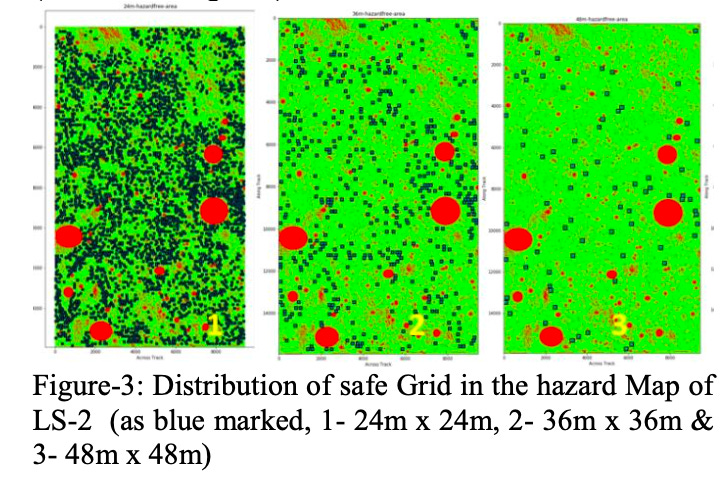
While these appear to be the standard criteria for ISRO’s landing site evaluations, the approach for Chandrayaan-3 — which landed much further north at 69.37°S, 32.35°E (between Manzinus U and Boguslawsky M craters) — was notably more elaborate. For CH3, ISRO evaluated a much larger 4 km × 2.4 km landing zone and applied a multi-grid assessment at three scales: 24 m × 24 m, 36 m × 36 m, and 48 m × 48 m (Amitabh et al., LPSC 2023, #1037). The winning site (LS-2) had 3,901 safe 24 m grids across the full zone.
The reason for this multi-scale approach was operational, not just analytical. CH3’s Vikram lander carried an onboard Hazard Detection and Avoidance (HDA) system (Suresh & Amitabh, LPSC 2024, #2250) that worked in two modes. In 3D mode, a camera image captured during hovering at ~150 m altitude was matched against a pre-stored OHRC orthoimage to localize the lander’s position within the 4 km × 2.4 km zone.
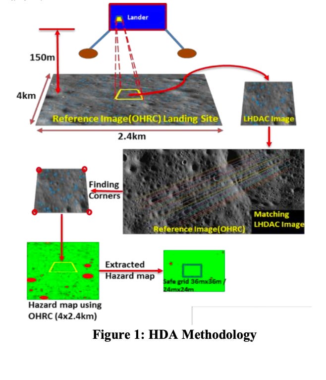
Once localized, the lander extracted the corresponding region from a pre-uploaded binary hazard map — prepared at 4 m grid spacing from the OHRC DEM — and searched for the nearest safe 24 m × 24 m grid to divert to if its nadir point was unsafe.
In 2D mode (a salvage option), the lander computed a hazard map in real-time from the descent camera image alone. The hazard map marked grids as unsafe based on four criteria: craters > 1.2 m, boulders > 0.32 m, slope > 10°, and shadow at the time of landing.
Additional mission constraints — Earth-Moon radio communication visibility and continuous illumination for 14 days — were also factored in. The multi-grid evaluation at 48 m, 36 m, and 24 m scales ensured that safe zones existed at multiple footprint sizes, giving the HDA system viable divert options regardless of where the lander ended up within its descent corridor. The landing area had been expanded from the original CH2-era 500 m × 500 m to 4 km × 2.4 km specifically to accommodate along-track and across-track trajectory dispersions during terminal descent.
For CH4, the landing box has shrunk to 1 km × 1 km with only the 24 m grid presumably tighter descent dispersions from improved navigation confidence gained during CH3’s successful landing.
I have the same Level-1 OHRC stereo imagery from ISRO’s PRADAN archive. The question: can I independently reproduce their analysis, and what can I learn about the methodology along the way?
The short answer: the DEM checks out, the alignment to LOLA reveals a 4.8 km offset that is entirely expected (which I realised later), and reverse-engineering the hazard classification turns out to be more interesting than I anticipated. In this post, I cover the DEM generation, LOLA alignment, and the first criterion — slope analysis. The full multi-criteria hazard map is a work in progress.
The Data
A note on the paper: the acquisition date is listed as November 2025, but the orbit numbers (23353/23354) correspond to November 2024 products in ISRO’s archive — a one-year typo.
The Figure-1 coordinate table also appears to have a site numbering swap (MM-3 and MM-4 coordinates are interchanged). They matter if you’re trying to reproduce the work programmatically, but they don’t undermine the science.
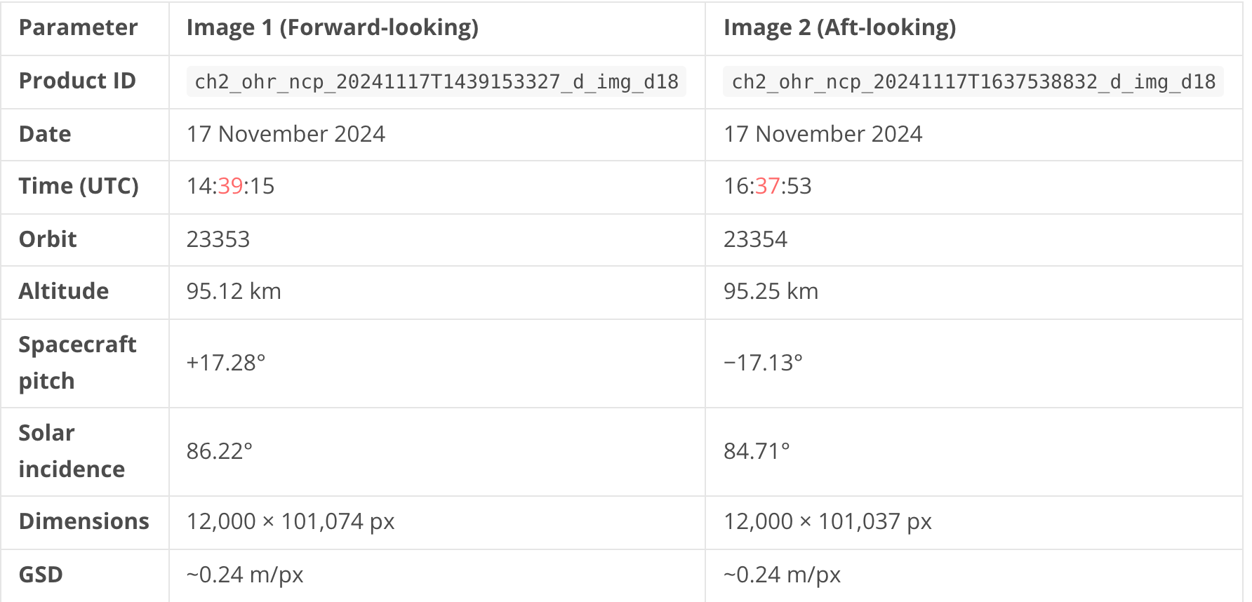
The stereo pair for MM-4 was acquired on consecutive orbits with opposite spacecraft pitch angles — +17.28° (forward-looking) and −17.13° (aft-looking) — producing a 36.89° convergence angle across a 63.7 km baseline. Both images were captured from ~95 km altitude at ~0.24 m/px ground sample distance, covering nearly identical swaths of 12,000 × ~101,000 pixels each. Solar incidence angles of 84–86° mean the sun was only 4–6° above the horizon, casting long shadows that enhance visual boulder detection but degrade stereo correlation in shadowed terrain.
The images come from Chandrayaan-2’s OHRC — the same camera I used for my previous DEM at the Chandrayaan-3 landing site. Quick specs:
Detector: 12,000-pixel TDI line array, 5.2 µm pitch
Focal length: 2080 mm
GSD: ~0.24 m/px (varies slightly with altitude)
Spectral band: 450–800 nm panchromatic
The catch: solar incidence is 84–86°. The sun is barely 4–5° above the horizon. Every surface feature throws a long, dramatic shadow — great for spotting boulders visually, terrible for stereo matching where those shadows leave no texture to correlate.
Building the High Resolution Elevation Map
I’ve covered the full pipeline in my previous post, so I’ll focus on the key numbers here.

The pipeline is the same: ISIS for ingestion and SPICE initialization, CSM camera models via a custom ISD generator, ASP for bundle adjustment, stereo correlation, and DEM generation.
Bundle adjustment was the most time-consuming step at ~9 hours, dominated by interest point matching on the full uncropped 12,000 × 101,000 pixel strips. 578k interest points were detected per image, filtered down to ~115k matches after outlier removal, with 10,000 used for the actual optimization. The solver converged in 21 iterations, reducing cost by 97.8% (14,203 → 308) with a final mean reprojection error of 0.31 pixels.
Stereo correlation used ASP’s MGM (More Global Matching) algorithm via parallel_stereo. The first pass with a 1-hour correlation timeout completed 275 of 296 tiles. A second pass at 2 hours recovered 12 more, leaving 9 tiles failed — all in deep shadow zones at strip edges where 84–86° solar incidence leaves no texture to correlate. ISRO’s in-house software handles these regions; ASP’s MGM doesn’t. The gaps are at the margins, not in the landing site area.
DEM generation with point2dem produced a 26,366 × 77,340 pixel grid at 0.289 m/px (auto-computed by ASP), spanning ~7.6 × 22.3 km with an elevation range of 4,729–5,618 m. Valid pixel coverage is 32.4% of the full grid — low because most of the grid falls outside the stereo overlap, but the overlap region itself has near-complete coverage.
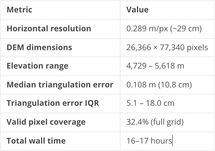
The 10.8 cm median triangulation error is excellent — well below a single pixel of GSD. For a 29 cm DEM built from ~95 km altitude with challenging 85° solar incidence, that’s right where it should be.
I also spent an unreasonable number of iterations matching ISRO’s color DEM palette — a non-standard ramp from teal through brown and red to pink-white, with unevenly spaced transitions — a Vanity project, but satisfying.
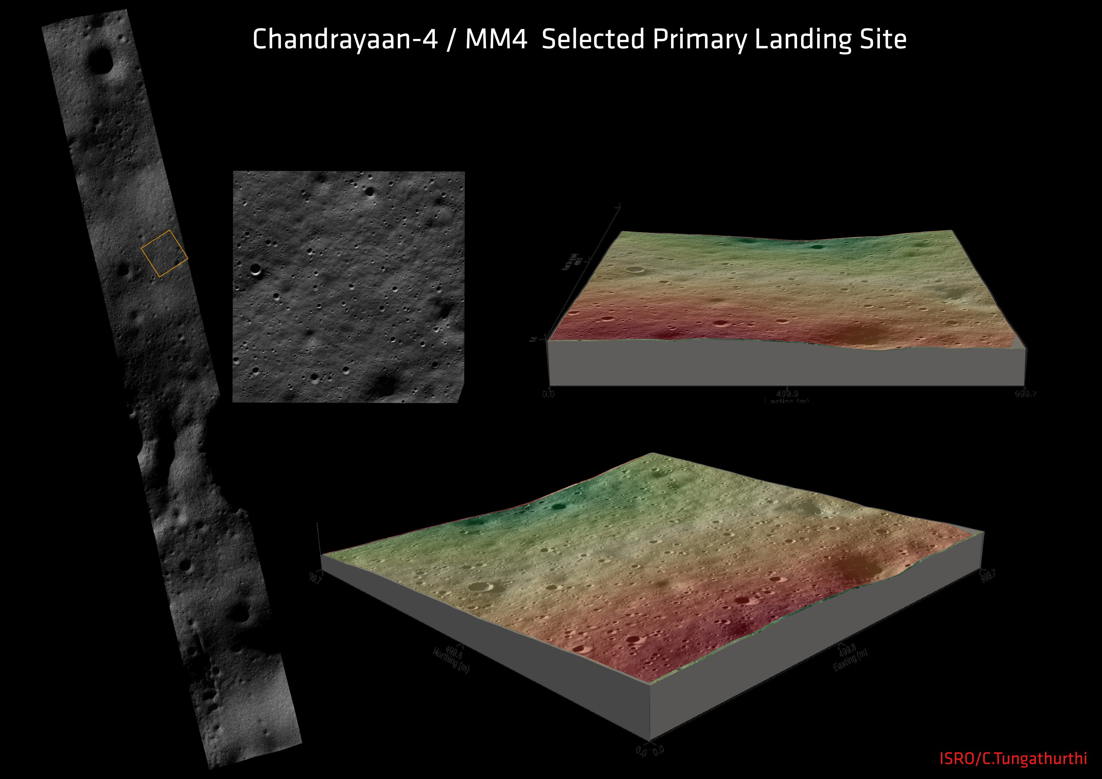
The Result: a 29cm elevation map
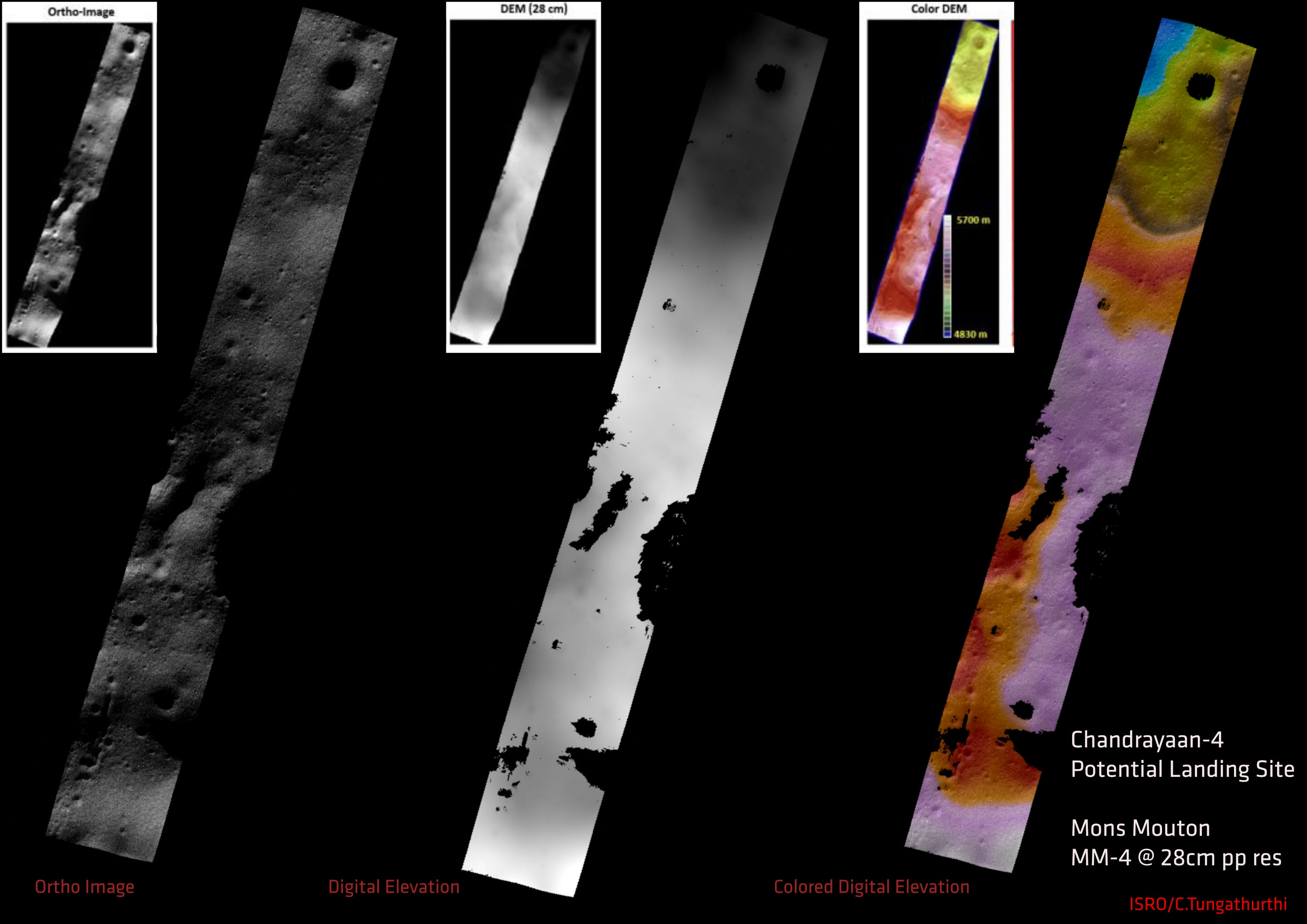
The orthoimage is the left stereo image reprojected onto the DEM surface — a map-projected view as if looking straight down, with terrain distortion removed. The grayscale DEM encodes elevation as brightness (white = high, dark = low), covering only the stereo overlap region where both images had matching texture. The colour DEM applies a palette across the 4,830–5,700 m elevation range to make topographic features visually distinct — the large dark crater near the top of the strip and the broad plateau of Mons Mouton are immediately apparent.


The black gaps in the DEM are shadow voids — regions where stereo correlation failed entirely. At 84–86° solar incidence, the sun is barely 4–6° above the horizon. Crater walls, ridges, and even modest undulations cast shadows that can stretch 10× the feature height. In these shadowed pixels, both stereo images record near-zero DN values with no texture for the correlator to match, producing no disparity and no 3D points.
These gaps are concentrated at strip edges and inside deep craters — not in the MM-4 landing site area. Of 296 stereo tiles, 9 failed even with a 2-hour correlation timeout, all in shadow-dominated regions.
Interestingly, ISRO’s published DEM and colour relief products show no such gaps — the coverage appears seamless even through shadowed terrain. The most likely explanation is algorithmic: ISRO’s OPTIMUS which almost certainly includes shadow-aware interpolation or multi-pass gap-filling as part of the production pipeline. ASP’s MGM correlator, by contrast, is conservative — if it can’t find a confident match, it reports no data rather than guessing.
ISRO may also leverage the slight difference in solar geometry between the two acquisitions (~1.5° change in solar incidence over the ~2 hour gap between orbits), using the image with marginally better shadow illumination to fill regions that are fully dark in the other. A third possibility is that ISRO applies shape-from-shading (photoclinometry) within shadow zones, using the faint secondary illumination from earthshine or terrain-scattered light to recover surface shape where stereo fails. Whatever the method, the gap-free result is a production pipeline advantage — though it’s worth noting that interpolated or photoclinometry-derived elevations in shadow zones carry higher uncertainty than stereo-derived values in well-lit terrain.
At this stage, the strip’s absolute position on the Moon is offset by ~4.8 km from its true location due to SPICE ephemeris errors. The internal geometry is accurate (10.8 cm triangulation error), but the whole strip needs to be shifted into place — which is what LOLA alignment does in the next section.
LOLA Alignment: The 4.8 km Surprise
Why align — Solving the coordinate misunderstanding
ISRO’s published MM-4 coordinate (-84.289°, 32.808°) fell in a nodata gap in my original (pre-alignment) DEM. After the 4.8 km northward shift: 100% valid coverage at that location. The coordinate was always correct — my DEM was just offset.
This also resolved the “coordinate mystery” from my first draft. The ~4 km discrepancy between the published coordinate and where I’d found the best statistical match? That was the alignment offset. Once the DEM is in the right place, the published coordinate lands exactly where it should.
SPICE camera models — the spacecraft position and pointing data used to build the sensor model — carry systematic errors. The DEM is geometrically correct internally (triangulation error: 10.8 cm), but its absolute position on the Moon will be offset, and this is expected. Every planetary data product built from orbital imagery has this problem until it is tied to a known independent reference. What “offset” really means here is that the coordinates in my DEM don’t agree with the coordinates in any other dataset — LOLA, LROC, even ISRO’s own published site locations. The terrain is right; the address is wrong. Alignment fixes the address.
Choosing the reference
The standard reference for absolute lunar positioning is LOLA — the Lunar Orbiter Laser Altimeter on LRO — which provides the definitive elevation reference for the Moon. In practice, most alignment work uses LOLA-derived gridded products known as “LDEMs” rather than raw altimetry tracks.
The product I used: LDEM_83S_10MPP_ADJ.TIF (Barker et al., 2023 Planet. Sci. J., 4, 183) a 10 m/px gridded DEM covering 83°S to the pole in south polar stereographic projection.
This matters because for my CH3 (Chandrayaan-3 landing site) alignment (arXiv:2602.14993) , I used hand-gridded LOLA RDR point shots — RDR being “Reduced Data Record,” the individual laser altimetry returns with latitude, longitude, and elevation for each pulse, as opposed to the gridded LDEM which interpolates millions of these returns into a continuous surface. The result was mediocre: 42 m median error. Switching to the official gridded LDEM product turned out to be 27× more accurate. The whole process of selecting references, running iterative alignment, and validating results gets tedious — in my previous post I’ve explained the methodology in detail. For now, the key is choosing a reference product that actually covers your regionof interest at sufficient resolution. This is where QuickMap comes in extremely handy — it lets you browse available data products and check coverage before committing to a reference.
Alignment
Step 1: Reproject both DEMs to the same CRS at 10 m. My DEM lives in an oblique stereographic projection; LOLA in south polar stereo. I reprojected mine into LOLA’s CRS at 10 m resolution.
Step 2: Translation-only ICP. First pass — just find the bulk shift, no rotation.
Initial median error: 175 m
Final median error: 15.7 m
Translation: 4,806 m, almost entirely northward
A 4.8 km offset. That’s large but not surprising — SPICE ephemeris errors of several kilometres are typical for lunar orbiters without ground control points, as explained earlier.
Step 3: Rigid refinement. Point-to-plane ICP seeded with the translation, now allowing rotation.
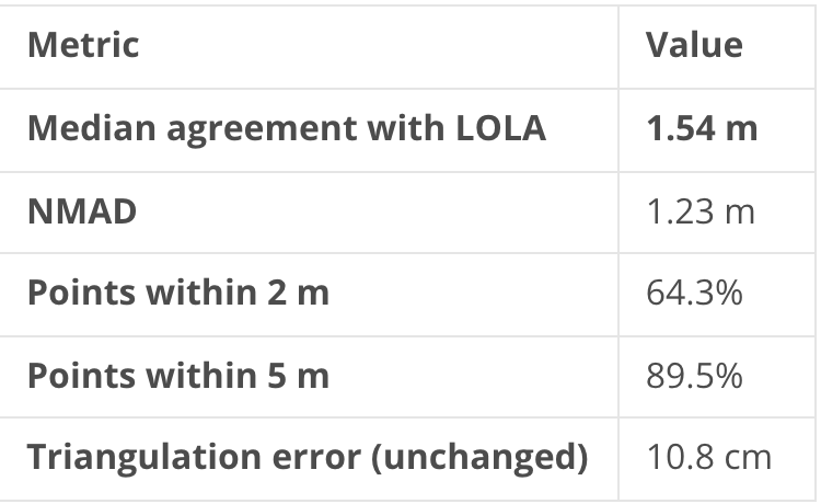
Initial: 13 m → Final: 1.54 m median
Rotation: 0.18°
Converged in 7 iterations
Step 4: Apply to full-resolution point cloud. The ICP was done at 10 m resolution for speed. Now apply the same rigid transform to the original ~0.3 m point cloud, then regenerate the DEM.
The rigid transform preserves internal geometry perfectly — triangulation error is identical before and after alignment.
The full alignment process is non-trivial and involves several careful decisions about reference selection, convergence criteria, and transform direction (I’ve documented the methodology in detail in my previous post). I’ve condensed it here to the numbers that matter — because for everything that follows, one number matters most: 1.54 m. That tells me the aligned DEM and orthoimage agree with the global LOLA reference to within 1.54 metres (!!) on average. That is an exceptionally good alignment — it means I can overlay my 29 cm products on any other lunar dataset and trust that features line up to within a couple of metres.
here you can see this clearly:
I’m refining this pipeline as I learn new things — each site I process teaches me something about reference selection, convergence behaviour, or edge cases. I’ve published my findings, methodology, results, and validations in a preprint:
Geodetically Anchored 0.30m Digital Elevation Model of the Chandrayaan-3 Vikram Landing Site from Chandrayaan-2 Orbital High Resolution Camera (OHRC) Stereo Imagery (Tungathurthi, 2025, preprint here )
and a formal journal submission is in preparation.
There’s no publicly available end-to-end guide for aligning CH2 OHRC products to LOLA, and it shouldn’t require the number of iterations it took me to get here.
The Potential Landing site
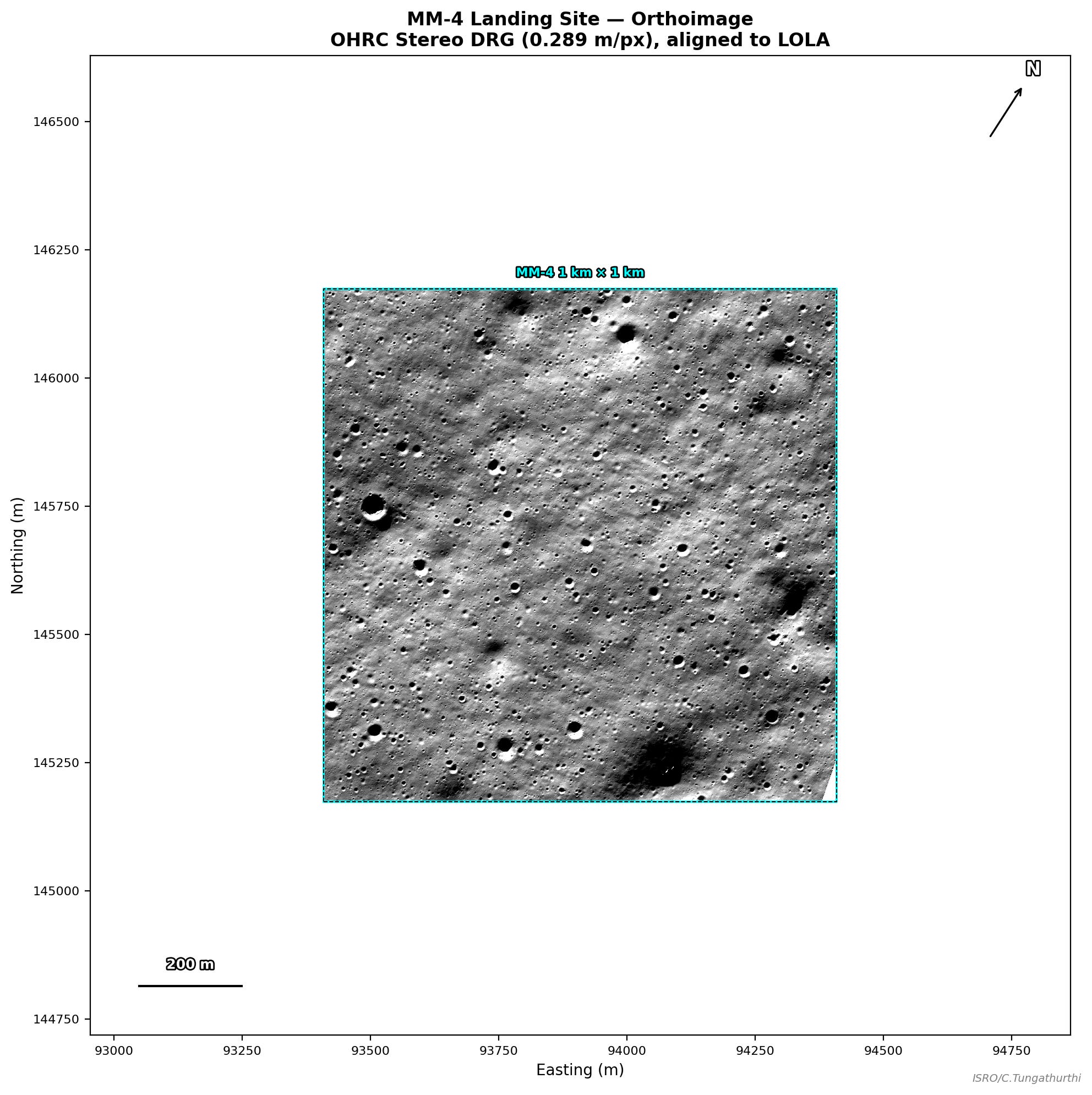
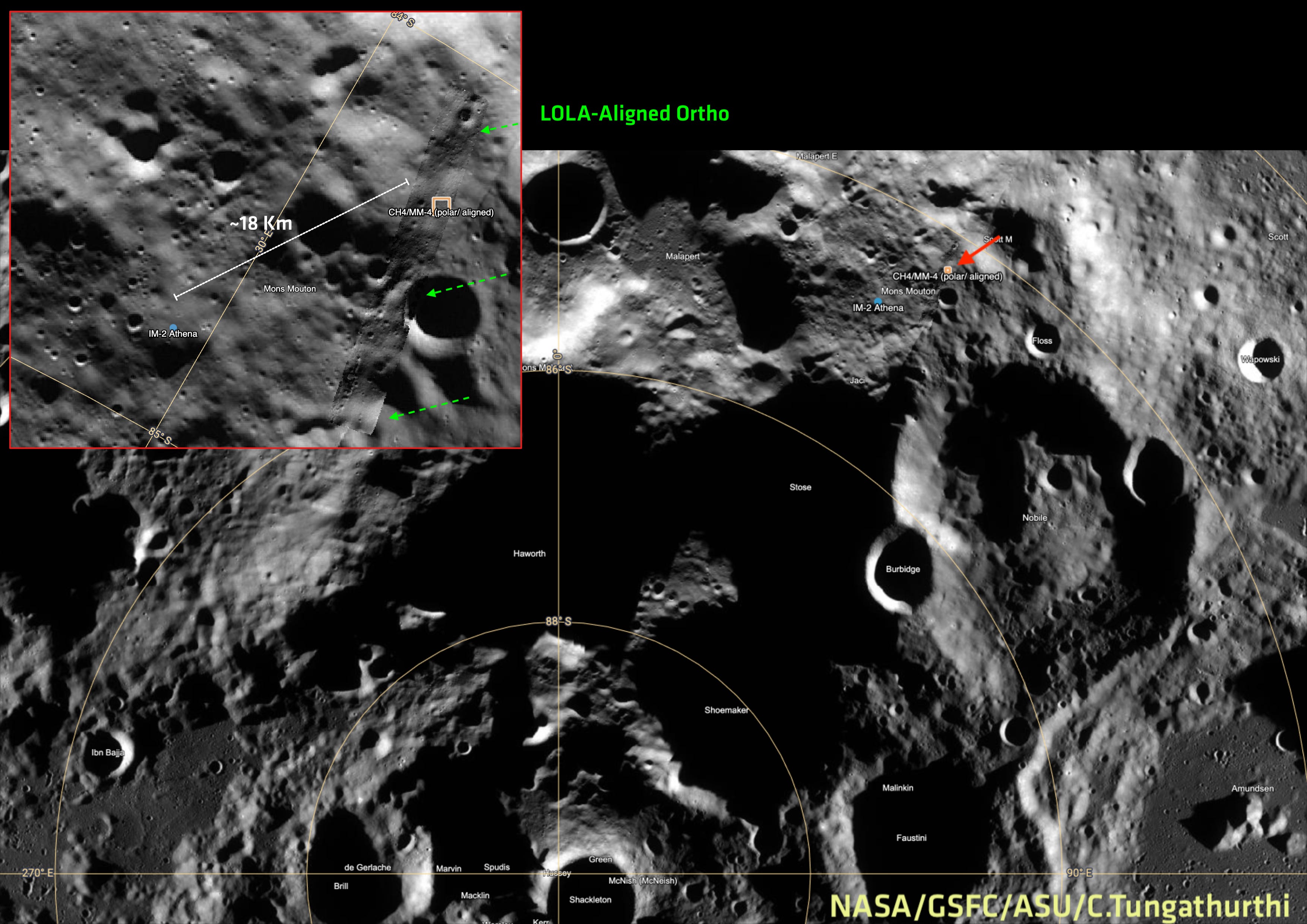
With the aligned DEM in hand, I can finally do what I set out to do: draw a 1 km × 1 km box at ISRO’s published coordinates (-84.289, 32.808)and examine the terrain.
ISRO’s LPSC abstract identifies MM-4 as the preferred site and provides a coordinate for the selected 1 km × 1 km landing area within it. This is the area within which the lander must touch down — significantly smaller than Chandrayaan-3’s 4 km × 2.4 km landing zone, reflecting tighter descent dispersions. After LOLA alignment, this coordinate falls squarely within high-quality DEM coverage — 100% valid pixels, no shadow gaps. The landing box sits on the relatively flat plateau of
Mons Mouton, flanked by small craters and gentle undulations, with an elevation range of about 100 metres across the full kilometre.
Box orientation matters
One subtlety I didn’t appreciate initially: the 1 km × 1 km box is defined with respect to ISRO’s south polar stereographic projection (centred at 90°S). My DEM uses oblique stereographic centred on the strip (lat₀ = −84.2°). A box that is axis-aligned in polar stereo is rotated ~33° relative to a box axis-aligned in my oblique stereo — because at longitude ~33°E, the polar stereo grid axes point in a different direction than the oblique stereo grid axes.
Both boxes are centred on the same latitude/longitude. But they cover different pixels due to the rotation, so the statistics differ slightly. When comparing with ISRO, you have to match their CRS.
Comparing with ISRO’s stats
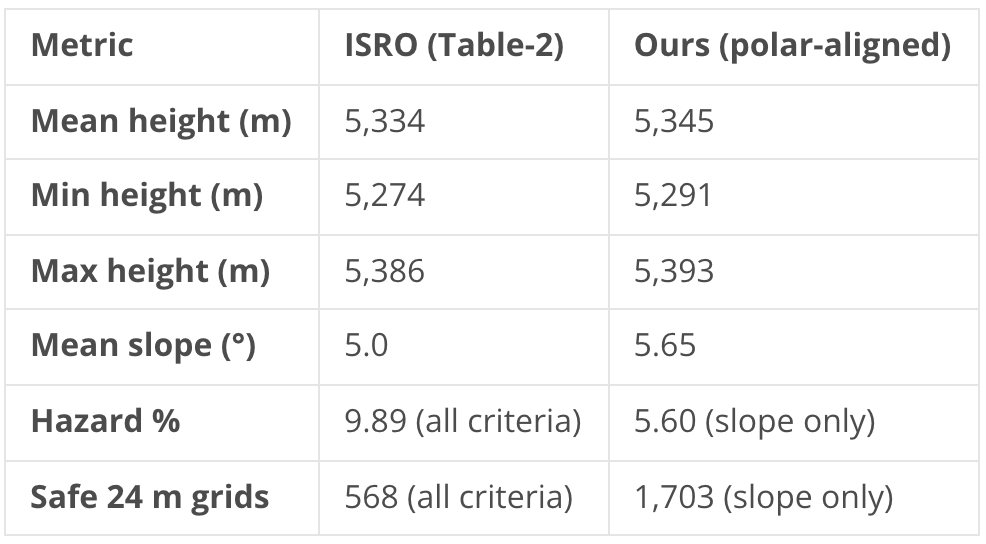
The ~10 m elevation offset is the LOLA alignment residual — a 1.54 m median means some areas are a few metres higher, others lower, and the mean offset at this particular location happens to be around 10 m. The slope difference (5.0° vs 5.65°) is consistent with different DEM resolutions and processing algorithms: our finer 0.289 m grid resolves more micro-terrain than ISRO’s 0.32 m grid, which slightly inflates the mean slope.
Hazard Mapping: The First Criterion — Slope
The first and most fundamental criterion in ISRO’s hazard classification is slope: any terrain steeper than 10° is flagged as unsafe. This is a hard engineering constraint — the lander’s legs and descent guidance are designed to handle up to 10° of local tilt at touchdown.
The most telling comparison is the safe grid count: 1,703 vs 568. Our count is higher because we’re only applying the slope criterion. ISRO applies all six criteria — slope, boulders, craters, illumination, shadow duration, and grid distribution. Additional criteria can only remove grids, never add them. So 1,703 > 568 is exactly correct: slope is a permissive filter at this site, and the other criteria — particularly illumination — do most of the heavy lifting.
The remaining criteria — boulder detection, crater mapping, illumination modelling, shadow duration, and grid distribution — are where the analysis gets genuinely difficult. Illumination in particular requires ray-tracing over a full lunar year at a latitude where the sun never climbs above 7°, and no public product exists at sufficient resolution for this site. In the next post, I’ll tackle these remaining criteria and attempt to recreate the full multi-criteria hazard map to compare directly with ISRO’s published Figure 6.
The foundation is solid. The interesting work is ahead.
Putting It All Together: 3D Terrain Mapping
To get a sense of what the lander will actually face, here’s the aligned DEM draped with the orthoimage and rendered as a 3D terrain slab from six perspectives. The elevation colour ramp (green = low, red = high) is blended with the orthoimage at 45% opacity to preserve surface texture — craters, boulder shadows, and micro-terrain are all visible alongside the elevation gradient.
The 1 km × 1 km landing box spans an elevation range of ~103 m (Δ = 103 m). The terrain is broadly flat with a gentle northward slope, punctuated by small craters and subtle ridges. From the bird’s-eye view, the scale of the site relative to individual craters becomes clear — most hazardous features are well under 50 m across. From the low-angle views, you can appreciate why slope matters: even modest undulations become significant when viewed at the 4–6° sun angles this site experiences.
Conclusion
Starting from the same Level-1 OHRC stereo imagery available on ISRO’s PRADAN portal, I’ve independently produced a 29 cm DEM with 10.8 cm triangulation error, aligned it to the global LOLA reference to within 1.54 m, and validated the first of ISRO’s six hazard criteria against their published numbers. The elevation statistics agree to within the alignment residual. The slope analysis confirms that terrain steepness alone is a permissive filter at MM-4 — 97% of 24 m grids pass —meaning the other five criteria do the real work of narrowing 1,703 slope-safe grids down to ISRO’s 568.
The remaining criteria — boulder detection, crater mapping, illumination modelling, shadow duration, and grid distribution — are where the analysis gets genuinely difficult. Illumination in particular requires ray-tracing over a full lunar year at a latitude where the sun never climbs above 7°, and no public product exists at sufficient resolution for this site. In the next post, I’ll tackle these remaining criteria and attempt to recreate the full multi-criteria hazard map.
The data is public. The tools are open-source. The methodology is published. ISRO’s numbers are there to be checked against — anyone should be able to verify them independently. That’s the point.
All processing done with open-source tools: ISIS 9.0.0, ALE 0.11.0, ASP 3.6.0, GDAL, and Python. Raw data from ISRO’s PRADAN portal. Full pipeline methodology published in Tungathurthi (2025).
~FIN